Boulariah O; Mikhailov PA; Longobardi A; Elizariev AN; Aksenov SG

doi:10.19637/j.cnki.2305-7068.2021.02.008

doi: 10.19637/j.cnki.2305-7068.2021.02.008

^1, ,,
²,
¹,
²,
²

计量
- 文章访问数: 1412
- HTML全文浏览量: 596
- PDF下载量: 93
- 被引次数: 0
出版历程
- 收稿日期: 2020-11-02
- 录用日期: 2021-04-20
- 网络出版日期: 2021-08-04
- 刊出日期: 2021-06-28

Assessment of prediction performances of stochastic models: Monthly groundwater level prediction in Southern Italy

1.
Department of Civil Engineering, University of Salerno, Via Giovanni Paolo II, 123, 84084, Italy
2.
Ufa State Aviation Technical University, 450000, Russian Federation

More Information

Corresponding author: oboulariah@unisa.it

摘要

- /
- /
- /
- /
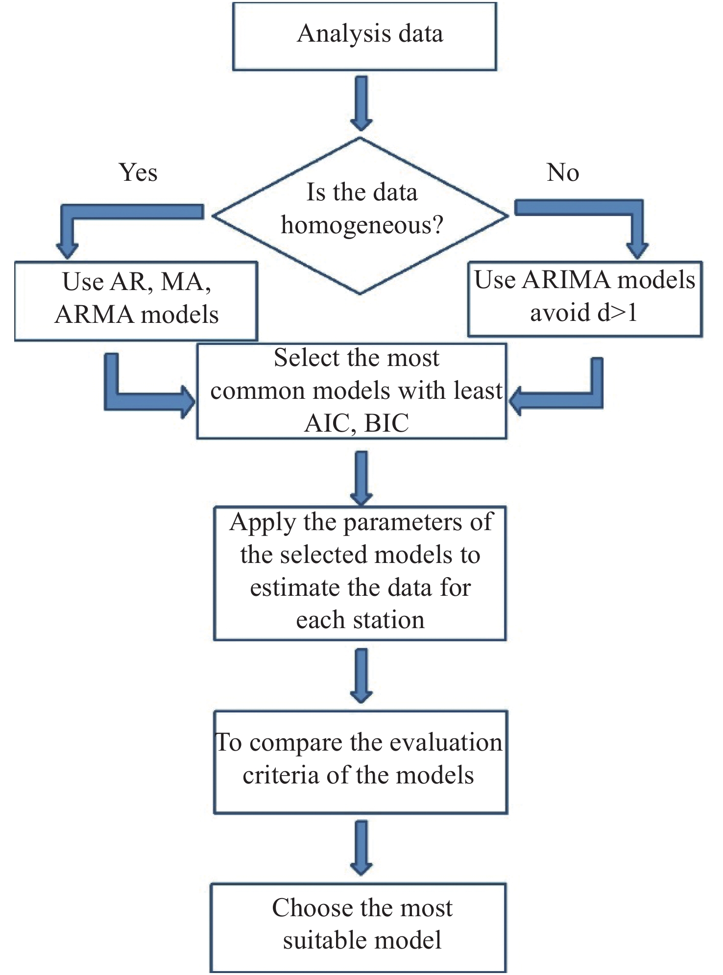
Abstract: Stochastic modelling of hydrological time series with insufficient length and data gaps is a serious challenge since these problems significantly affect the reliability of statistical models predicting and forecasting skills. In this paper, we proposed a method for searching the seasonal autoregressive integrated moving average (SARIMA) model parameters to predict the behavior of groundwater time series affected by the issues mentioned. Based on the analysis of statistical indices, 8 stations among 44 available within the Campania region (Italy) have been selected as the highest quality measurements. Different SARIMA models, with different autoregressive, moving average and differentiation orders had been used. By reviewing the criteria used to determine the consistency and goodness-of-fit of the model, it is revealed that the model with specific combination of parameters, SARIMA (0,1,3) (0,1,2) ₁₂, has a high R² value, larger than 92%, for each of the 8 selected stations. The same model has also good performances for what concern the forecasting skills, with an average NSE of about 96%. Therefore, this study has the potential to provide a new horizon for the simulation and reconstruction of groundwater time series within the investigated area.
- Groundwater level forecast /
- Stochastic modelling /
- Southern Italy /
- Seasonality /
- Homogeneity

HTML全文

Figure 1. Flowchart of applied methodology for forecasting time series

下载: 全尺寸图片幻灯片

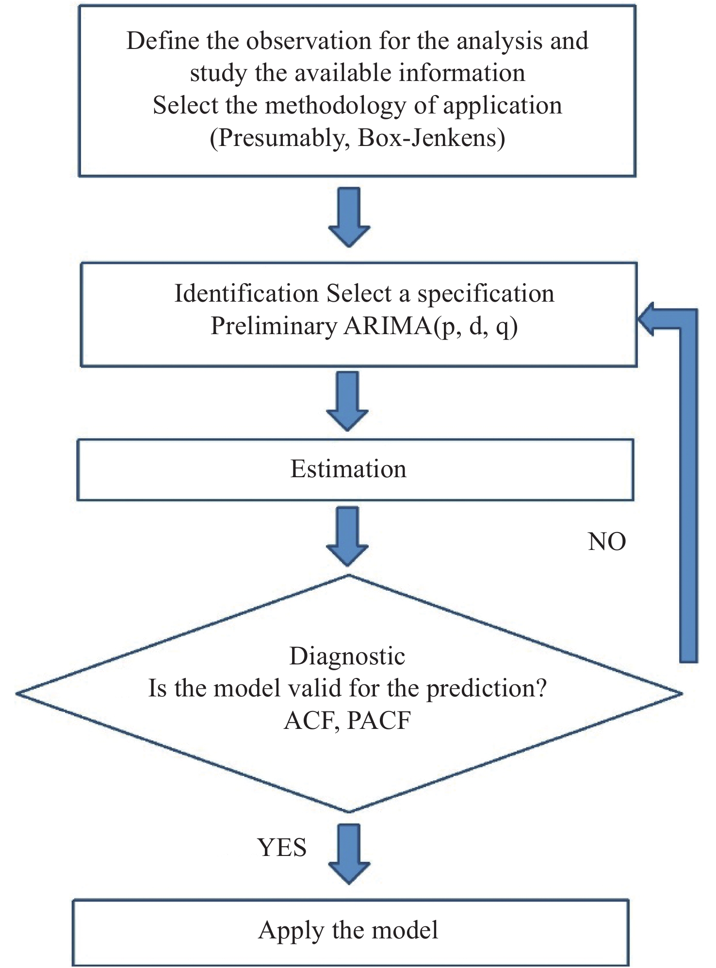
Figure 2. ARIMA model prediction method (Chatfield et al.1973)

下载: 全尺寸图片幻灯片

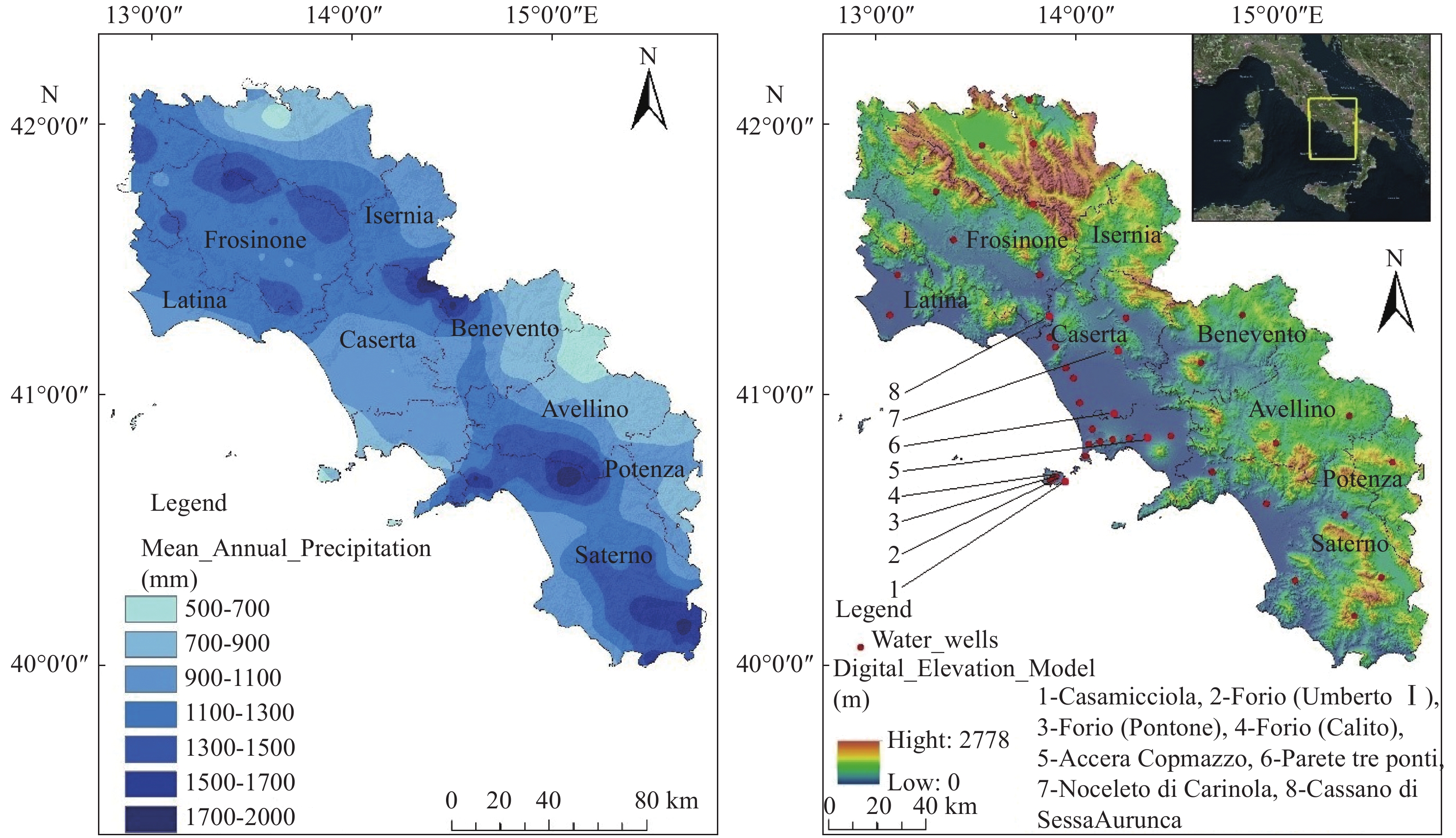
Figure 3. Digital elevation model with location of water wells (right panel) and mean annual precipitation (left panel) in the study area

下载: 全尺寸图片幻灯片

Figure 4. Predicted and observed values of the ground water level.

下载: 全尺寸图片幻灯片

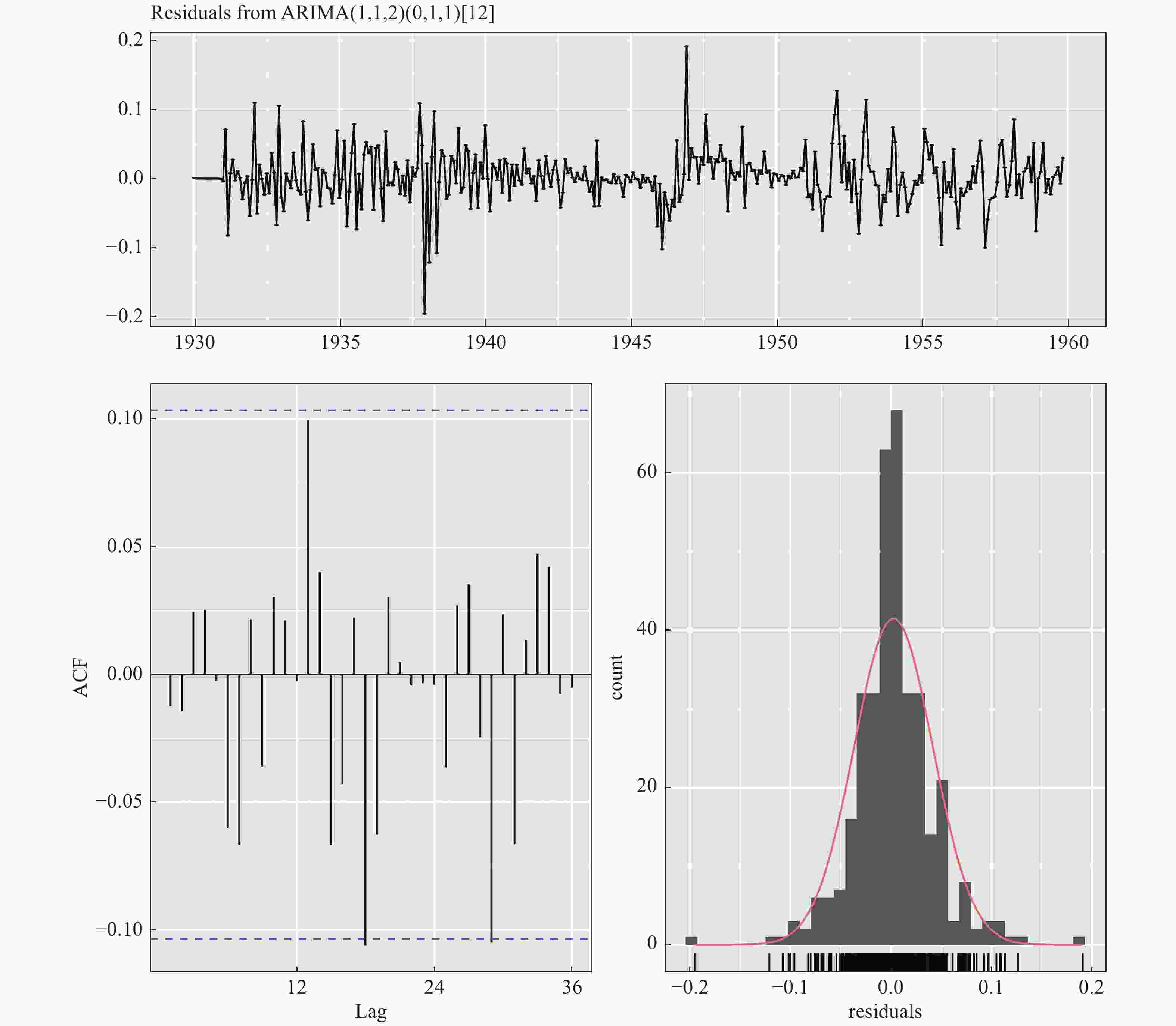
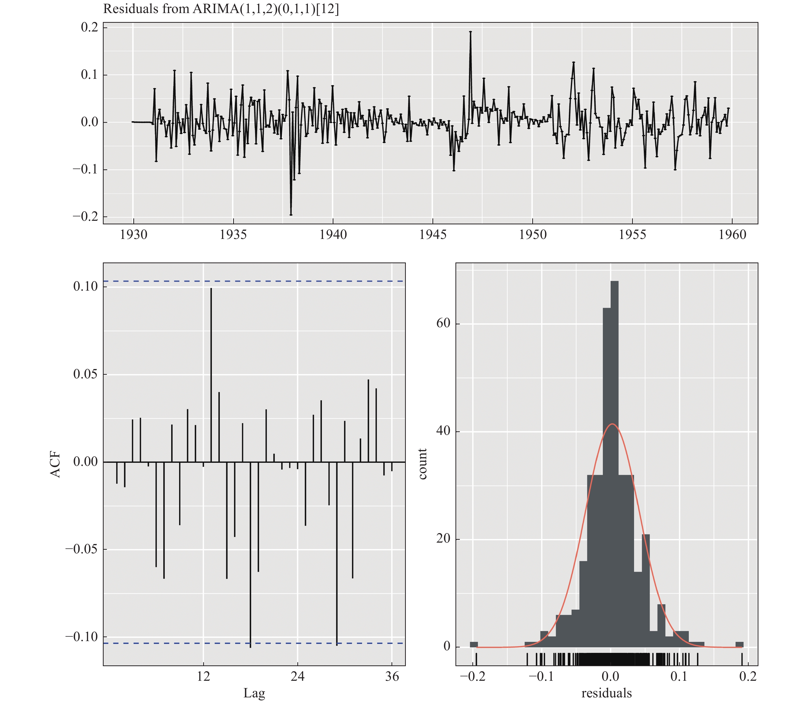
Figure 5. Autocorrelation function graph for the residues of the SARIMA model (1,1,2) (0,1,1)₁₂

下载: 全尺寸图片幻灯片

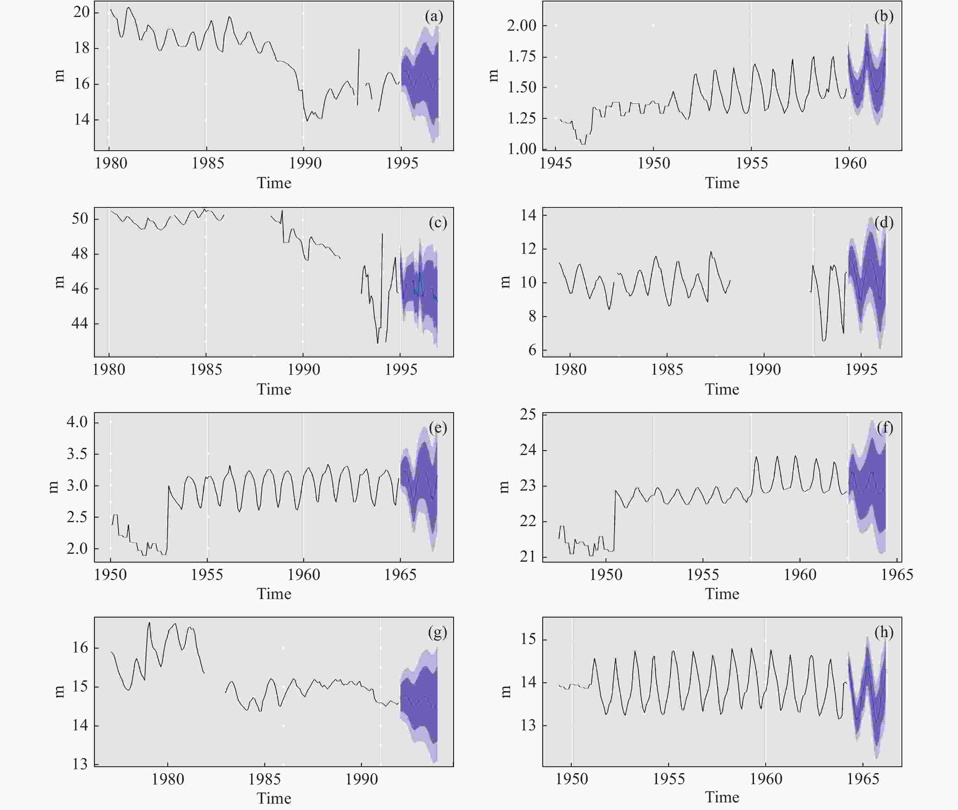
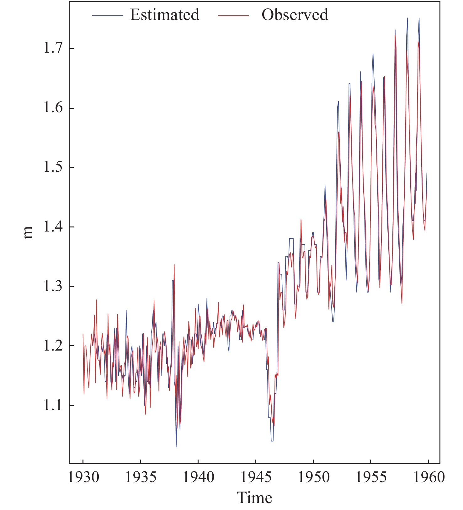
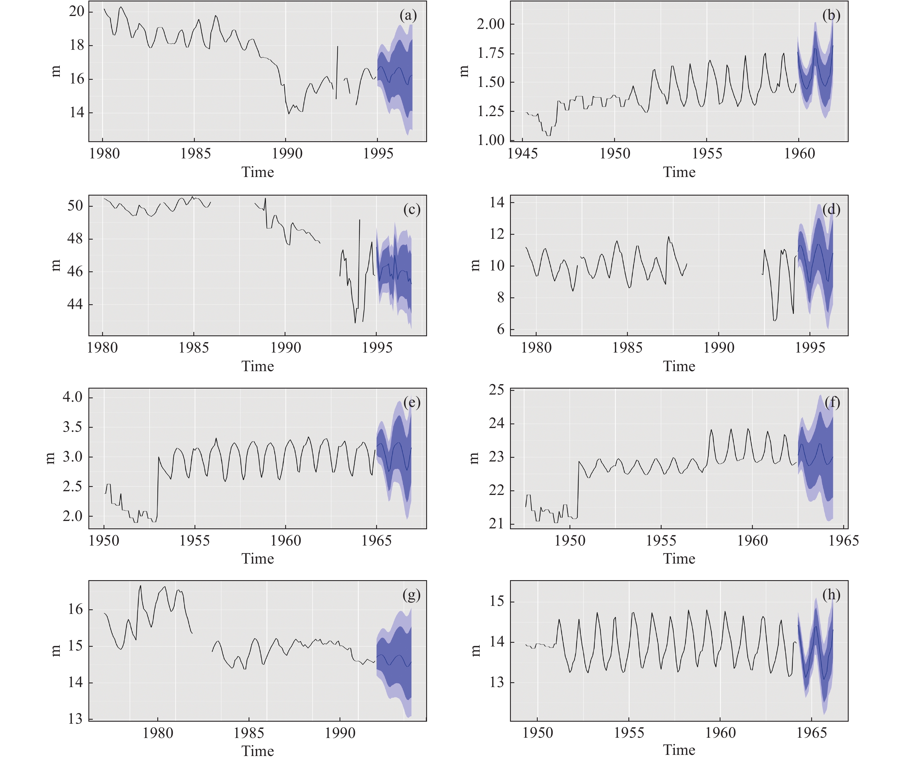
Figure 6. Forecasting using SARIMA(0,1,3)(0,1,2)₁₂; (a) Acera Capomazzo, (b) Casamicciola, (c) Cassano di Sessa Aurunca, (d) Forio(Calitto), (e) Forio(Pontone), (f) Forio(Umberto I), (g) Nocelleto di Carinola, (h) Parete(tre ponti) scrivi cosa sono le fasce colorate.

下载: 全尺寸图片幻灯片

Table 1. Forecasting models Results based on AIC and BIC criteria

Name of station	Parameters of model	AIC	BIC
Acera Capomazzo	(1,1,2)(0,1,2)₁₂	514.44	542.39
Casamicciola	(1,1,2)(0,1,1)₁₂	−1228.75	−1209.5
Cassano di Sessa Aurunca	(0,1,3)(0,1,2)₁₂	914.41	942.54
Forio(Calitto)	(1,1,2)(0,1,1)₁₂	607.55	630.75
Forio(Pontone)	(0,1,3)(0,1,2)₁₂	−571.39	−547.92
Forio(Umberto I)	(1,1,1)(0,1,1)₁₂	−39.8	−24.01
Nocelleto di Carinola	(1,1,1)(0,1,1)₁₂	−377.44	−309.26
Parete(tre ponti)	(1,1,2)(0,1,1)₁₂	−702.58	−682.21

下载: 导出CSV

Table 2. The comparison of different SARIMA models based on accuracy measures

	Parete (tre ponti)	Nocelleto di carinola	Forio (Umberto I)	Forio (Pontone)	Forio (Calitto)	Cassano di Sessa Aurunca	Casamicciola	Accera Copmazzo
SARIMA (0,1,3)(0,1,2)₁₂
NSE	0.944	0.996	0.920	0.949	0.985	0.999	0.932	0.984
MAE	0.065	0.110	0.131	0.067	0.217	0.255	0.026	0.214
RMSE	0.107	0.183	0.218	0.108	0.363	0.420	0.037	0.331
Pearson cоr.	0.971	0.935	0.960	0.974	0.962	0.930	0.965	0.983
MSE	0.011	0.032	0.047	0.011	0.121	0.176	0,001	0.109
d	0.999	0.999	0.999	0.999	0.999	0.999	0.999	0.999
BIAS$	−0.026	0.027	−0.006	−0.012	−0.046	−0.045	0.036	0.003
MSDE	4.7E-04	4.3E-06	1.5E-05	3.1E-09	0.006	0.101	2.2E-06	0.016
R²	0.944	0.874	0.922	0.949	0.9257	0.865	0.932	0.967
AIC	−678.64	−321.22	−36.87	−571.61	625.55	914.41	−1203.63	532.08
BIC	−654.2	−294.18	−13.18	−547.92	652.85	941.39	−1180.55	559.97
SARIMA (1,1,2)(0,1,1)₁₂
NSE	0.943	0.996	0.920	0.947	0.689	0.999	0.930	0.984
MAE	0.064	0.109	0.129	0.068	0.529	0.255	0.026	0.211
RMSE	0.108	0.182	0.218	0.110	1625774	0.422	0.037	0.329
Pearson cor.	0.971	0.934	0.960	0.973	0.553	0.929	0.964	0.983
MSE	0.012	0.032	0.047	0.012	0.419	0.178	0.001	0.107
d	0.999	0.999	0.999	0.999	0.999	0.999	0.999	0.999
BIAS$	−0.018	0.032	−0.0088	−0.013	−2.340	−0.046	−0.117	0.057
MSDE	0.0001	2.6E-06	1.3E-05	3.1E-09	0.198	0.106	2.2E-06	0017
R²	0.943	0.873	0.921	0.948	0.306	0.863	0.931	0.967
AIC	−702.58	−327.03	−37.95	−562.72	607.55	920.63	−1226.74	519.45
BIC	−682.21	−304.5	−18.2	−542.97	630.3	943.12	−1207.5	542.69
SARIMA (1,1,2)(0,1,1)₁₂
NSE	0.943	0.996	0.920	0.946	0.985	0.999	0.940	0.984
MAE	0.063	0.110	0.129	0.069	0.219	0.257	0.024	0.212
RMSE	0.108	0.183	0.218	0.111	0.365	0.424	0.034	0.330
Pearson cor.	0.971	0.934	0.960	0.973	0.962	0.928	0.970	0.983
MSE	0,011	0.032	0.047	0.012	0.122	0.180	0.001	0.107
d	0.999	0.999	0.999	0.999	0.999	0.999	0.999	0.999
BIAS$	−0.018	0.033	−0.008	−0.013	−0.042	−0.047	0.048	0.061
MSDE	0,0001	2.4E-06	1.3E-05	3.1E-09	0.005	0.109	2.2E-06	0017
R²	0.943	0.873	0.921	0.947	0.862	0.862	0.941	0.967
AIC	−672.01	−327.44	−39.8	−561.6	629.36	924.5	−1194.32	518.6
BIC	−655.71	−309.41	−24	−545.8	647.56	942.491	−1178.931	537.19

下载: 导出CSV

Table 3. Statistical index values for the selected SARIMA model (0,1,3) (0,1,2)₁₂

	NSE	BIAS%	R²	d	r
Accera Copmazzo	0.98	0.003	0.96	0.99	0.98
Casamicciola	0.93	0.03	0.93	0.99	0.96
Cassano di Sessa Aurunca	0.99	−0.04	0.86	0.99	0.93
Forio Calitto	0.98	−0.04	0.92	0.99	0.96
Forio Pontone	0.94	−0.012	0.94	0.99	0.97
Forio Umberto I	0.92	−0.006	0.92	0.99	0.96
Nocelleto di carinola	0.99	0.02	0.87	0.99	0.93
Parete tre ponti	0.94	−0.02	0.94	0.99	0.97
Model Quality (Very good)	0.75< NSE<1.00	PBIAS<±10	0.75 < R²≤ 1.0	1	r > 0.7

下载: 导出CSV

参考文献(33)

Adamowski J. 2008. Development of a short-term river flood forecasting method for snowmelt driven floods based on wavelet and cross-wavelet analysis. Journal of Hydrology, 353: 247-266. doi: 10.1016/j.jhydrol.2008.02.013.

Ahn H, Salas J. 1997. Groundwater head sampling based on stochastic analysis. Water Resources Research, 33: 2769-2780. doi: 10.1029/97WR02187.

Balasmeh A, Babbar O, Karmaker T. 2019. Trend analysis and ARIMA modeling for forecasting precipitation pattern in Wadi Shueib catchment area in Jordan. Arabian Journal of Geosciences, 12: 27-27. doi: 10.1007/s12517-018-4205-z.

Boulariah O, Meddi M, Longobardi A. 2019. Assessment of prediction performances of stochastic and conceptual hydrological models: Monthly stream flow prediction in northwestern Algeria. Arabian Journal of Geosciences, 12: 792-792. doi: 10.1007/s12517-019-4847-5.

Chatfield C, Prothero DL. 1973. Box‐Jenkins seasonal forecasting: Problems in a case‐study. Journal of the Royal Statistical Society: Series A (General), 136(3): 295-315. doi: 10.2307/2344994.

Cleophas T, Zwinderman A. 2016. One-Sample Continuous Data (One-Sample T-Test, One-Sample Wilcoxon Signed Rank Test, 10 Patients). SPSS for Starters and 2nd Levelers: 3-6.

Faruk DÖ. 2010. A hybrid neural network and ARIMA model for water quality time series prediction. Engineering applications of artificial intelligence, 23(4), 586-594.

Hamilton J. 1994. Time series analysis. Princeton University Press. 1-820.

Jaiswal R, Lohani A, Tiwari H. 2015. Statistical Analysis for Change Detection and Trend Assessment and Climatological Parameters. Environmental Processes: 729-749.

Kumar KS, Rathnam EV. 2019. Analysis and prediction of groundwater level trends using four variations of Mann Kendall tests and ARIMA modelling. Journal of the Geological Society of India, 94: 281-289. doi: 10.1007/s12594-019-1308-4.

Longobardi A, Villani P. 2006. Seasonal response function for daily stream flow investigation. Physics and Chemistry of the Earth, 31: 1107-1117. doi: 10.1016/j.pce.2006.02.063.

Longobardi A, Van Loon A. 2018. Base flow index vulnerability to variation in dry spell length for a range of catchment and climate properties. Hydrological Processes, 32: 2496-2509. doi: 10.1002/hyp.13147.

Montgomery DC, Jennings CL, Kulahci M. 2015. Introduction to time series analysis and forecasting. John Wiley & Sons.

Mirzavand M, Ghazavi R. 2014. A stochastic modelling technique for groundwater level forecasting in an arid environment using time series methods. Water resources management, 29(4): 1315-1328. doi: 10.1007/s11269-014-0875-9.

Mirzavand M, Ghazavi R. 2015. A stochastic modelling technique for groundwater level forecasting in an arid environment using time series methods. Water resources management, 29(4): 1315-1328.

Mohammadi K, Eslami H, Dayani DS. 2005. Comparison of regression, ARIMA and ANN models for reservoir inflow forecasting using snowmelt equivalent (a case study of Karaj). Journal of Agricultural Science and Technology, 7: 17-30.

Mombeni H, Rezaei S, Nadarajah S, et al. 2013. Estimation of water demand in Iran based on SARIMA models. Environmental Modeling & Assessment, 18: 559-565.

Moriasi D, ARnoid G, Kuijk M, et al. 2007. Model evaluation guidelines for systematic quantification of accuracy in watershed simulations. Transactions of the ASABE, 50: 885-900. doi: 10.13031/2013.23153.

Nash J, Sutcliffe J. 1970. River flow forecasting through conceptual models part I — A discussion of principles. Journal of Hydrology, 10: 282-290. doi: 10.1016/0022-1694(70)90255-6.

Nunno FD, Granata F. 2020. Groundwater level prediction in Apulia region (Southern Italy) using NARX neural network. Environmental Research, 190: 110062. doi: 10.1016/j.envres.2020.110062.

Oikonomou PD, Alzraiee AH, Karavitis CA, et al. 2018. A novel framework for filling data gaps in groundwater level observations. Advances in Water Resources, 119: 111-124. doi: 10.1016/j.advwatres.2018.06.008.

Semiromi M, Koch M. 2019. Reconstruction of groundwater levels to impute missing values using singular and multichannel spectrum analysis: application to the Ardabil Plain, Iran. Hydrological sciences journal, 64: 1711-1726. doi: 10.1080/02626667.2019.1669793.

Singh J, Knapp H, Arnold J, et al. 2005. Hydrologic modeling of the Iroquois River watershed using HSPF and SWAT. J. American Water Resources Assoc, 41(2): 361-375. doi: 10.1111/j.1752-1688.2005.tb03741.x.

Suryanarayana C, Sudheer C, Mahammood V, et al. 2014. An integrated wavelet-support vector machine for groundwater level prediction in Visakhapatnam, India. Neurocomputing, 145: 324-335. doi: 10.1016/j.neucom.2014.05.026.

Takafuji E, Rocha M, Manzione R. 2019. Groundwater level prediction forecasting and assessment of uncertainty using SGS and ARIMA Models: A case study in the Bauru Aquifer System (Brazil). Natural Resources Research, 28: 487-503. doi: 10.1007/s11053-018-9403-6.

Valipour M, Banihabib M, Behbahani S. 2013. Comparison of the ARMA, ARIMA, and the autoregressive artificial neural network models in forecasting the monthly inflow of Dez dam reservoir. Journal of Hydrology, 476: 433-441. doi: 10.1016/j.jhydrol.2012.11.017.

Valipour M. 2013a. Increasing irrigation efficiency by management strategies: cutback and surge irrigation. ARPN Journal of Agricultural and Biological Science. 8(1):35-43.

Valipour M. 2013b. Necessity of irrigated and rainfed agriculture in the world. Irrigation & Drainage Systems Engineering. S9, e001.

Valipour M. 2012. Ability of Box-Jenkins models to estimate of reference potential evapotranspiration (A case study: Mehrabad Synoptic Station, Tehran, Iran). IOSR Journal of Agriculture and Veterinary Science, 1.5: 1-11.

Willmott C. 1981. On the validation of models. Physical Geography, 2: 184-194. doi: 10.1080/02723646.1981.10642213.

Willmott CJ, Matsuura K. 2005. Advantages of the mean absolute error (MAE) overthe root mean square error (RMSE) in assessingaverage model performance, 30, 79-82.

Young P. 1999. Nonstationary time series analysis and forecasting. Progress in Environmental Science, 1: 3-48.

Yang Q, Wang Y, Zhang J, et al. 2017. A comparative study of shallow groundwater level simulation with three time series models in a coastal aquifer of South China. Applied Sciences, 7: 689-698. doi: 10.3390/app7070689.

[1]	Ming-yang Li, Chao-zhu Li, Feng Dong, Peng Jiang, Yong-qiang Li2024: Groundwater level thresholds for maintaining groundwater-dependent ecosystems in northwest China: Current developments and future challenges, Journal of Groundwater Science and Engineering, 12, 453-462. doi: 10.26599/JGSE.2024.9280032
[2]	Stephen Pitchaimani V, Narayanan MSS, Abishek RS, Aswin SK, Jerin Joe RJ2024: Delineation of groundwater potential zones using remote sensing and Geographic Information Systems (GIS) in Kadaladi region, Southern India, Journal of Groundwater Science and Engineering, 12, 147-160. doi: 10.26599/JGSE.2024.9280012
[3]	Tian Nan, Chen Yue, Wen-geng Cao, En-lin Mu, Yang Ou, Zhen-sheng Lin, Wei Kang2023: Effective groundwater level recovery from mining reduction: Case study of Baoding and Shijiazhuang Plain area, Journal of Groundwater Science and Engineering, 11, 278-293. doi: 10.26599/JGSE.2023.9280023
[4]	Parisa Kazerani, Ali Naghi Ziaei, Kamran Davari2023: Determining safe yield and mapping water level zoning in groundwater resources of the Neishabour Plain, Journal of Groundwater Science and Engineering, 11, 47-54. doi: 10.26599/JGSE.2023.9280005
[5]	Edmealem Temesgen, Demelash Wendmagegnehu Goshime, Destaw Akili2023: Determination of groundwater potential distribution in Kulfo-Hare watershed through integration of GIS, remote sensing, and AHP in Southern Ethiopia, Journal of Groundwater Science and Engineering, 11, 249-262. doi: 10.26599/JGSE.2023.9280021
[6]	Yang Hui-feng, Meng Rui-fang, Bao Xi-lin, Cao Wen-geng, Li Ze-yan, Xu Bu-yun2022: Assessment of water level threshold for groundwater restoration and over-exploitation remediation the Beijing-Tianjin-Hebei Plain, Journal of Groundwater Science and Engineering, 10, 113-127. doi: 10.19637/j.cnki.2305-7068.2022.02.002
[7]	Chen She-ming, Liu Hong-wei, Liu Fu-tian, Miao Jin-jie, Guo Xu, Zhang Zhou, Jiang Wan-jun2022: Using time series analysis to assess tidal effect on coastal groundwater level in Southern Laizhou Bay, China, Journal of Groundwater Science and Engineering, 10, 292-301. doi: 10.19637/j.cnki.2305-7068.2022.03.007
[8]	Vinay Kumar Gautam, Mahesh Kothari, P.K. Singh, S.R. Bhakar, K.K. Yadav2022: Analysis of groundwater level trend in Jakham River Basin of Southern Rajasthan, Journal of Groundwater Science and Engineering, 10, 1-9. doi: 10.19637/j.cnki.2305-7068.2022.01.001
[9]	Kirlas Marios C2021: Assessment of porous aquifer hydrogeological parameters using automated groundwater level measurements in Greece, Journal of Groundwater Science and Engineering, 9, 269-278. doi: 10.19637/j.cnki.2305-7068.2021.04.001
[10]	Gao Fei, Liu Feng, Wang Hua-jun2021: Numerical modelling of the dynamic process of oil displacement by water in sandstone reservoirs with random pore structures, Journal of Groundwater Science and Engineering, 9, 233-244. doi: 10.19637/j.cnki.2305-7068.2021.03.006
[11]	Luong Van Viet2021: Effects of urbanization on groundwater level in aquifers of Binh Duong Province, Vietnam, Journal of Groundwater Science and Engineering, 9, 20-36. doi: 10.19637/j.cnki.2305-7068.2021.01.003
[12]	Nguyen Van Hoang2021: Determination of groundwater solute transport parameters in finite element modelling using tracer injection and withdrawal testing data, Journal of Groundwater Science and Engineering, 9, 292-303. doi: 10.19637/j.cnki.2305-7068.2021.04.003
[13]	Abdulrahman Th Mohammad, Qassem H Jalut, Nadia L Abbas2020: Predicting groundwater level of wells in the Diyala River Basin in eastern Iraq using artificial neural network, Journal of Groundwater Science and Engineering, 8, 87-96. doi: 10.19637/j.cnki.2305-7068.2020.01.009
[14]	JIANG Ti-sheng, QU Ci-xiao, WANG Ming-yu, SUN Yan-wei, HU Bo, CHU Jun-yao2017: Analysis on temporal and spatial variations of groundwater hydrochemical characteristics in the past decade in southern plain of Beijing, China, Journal of Groundwater Science and Engineering, 5, 235-248.
[15]	ZHOU Zhi-chao, WANG Ju, SU Rui, GUO Yong-hai, LI Jie-biao, JI Rui-li, ZHANG Ming, DONG Jian-nan2016: Study on the residence time of deep groundwater for high-level radioactive waste geological disposal, Journal of Groundwater Science and Engineering, 4, 52-59.
[16]	MA Luan, WANG Guang-cai, SHI Zhe-ming, GUO Yu-ying, XU Qing-yu, HUANG Xu-juan2016: Simulation of groundwater level recovery in abandoned mines, Fengfeng coalfield, China, Journal of Groundwater Science and Engineering, 4, 344-353.
[17]	XIA Ri-yuan2016: Groundwater resources in karst area in Southern China and sustainable utilization pattern, Journal of Groundwater Science and Engineering, 4, 301-309.
[18]	YANG Xiang-peng, ZHANG Fa-wang, CHEN Zhen, BI Xue-li, SHI Jian, ZHOU Li-xin, YANG Chen2015: Compiling distribution of karst in Southern China and Southeast Asia, Journal of Groundwater Science and Engineering, 3, 280-284.
[19]	Ramasamy Jayakumar2015: Groundwater level monitoring-importance global groundwater monitoring network, Journal of Groundwater Science and Engineering, 3, 295-305.
[20]	ZHANG Chuan-mian, GUO Xiao-niu, Richard Henry, James Dendy2015: Groundwater modelling to help diagnose contamination problems, Journal of Groundwater Science and Engineering, 3, 285-294.